Acoustic scene classification is the task where we try to classify a sound segment (e.g. 30 seconds long) to an acoustic scene, like airport, metro station, office, etc. We get a recording, we give it as an input to our acoustic scene classification method, and the method outputs the acoustic scene where this recording came from. To develop our method, we use a dataset of recordings of a list of acoustic scenes. When the method is ready, we can use it with any other recordings that can be classified to one of the acoustic scenes that our training data had. A known problem is the degradation of such methods when they are used with data recorded with different conditions than the ones used for training. 

Different conditions, usually, mean different acoustic channels (e.g. different recording devices). This difference introduces a mismatch between the conditions of the data that the method was trained on and the conditions of the data that the method encounters after training (e.g. at testing or deployment). The different conditions of the recordings are introducing the phenomenon known as dataset bias or domain shift. The act of tackling the domain shift phenomenon is called domain adaptation.

In our work entitled “Adversarial Unsupervised Domain Adaptation for Acoustic Scene Classification”, we present the first approach of domain adaptation for acoustic scene classification. To do so, we use one dataset recorded from a device (domain), device A, and data recorded from two other devices/domains, the B and C. All data are publicly available at the website of DCASE 2018, Task 1 (subtask B). Our approach is inspired by the Adversarial Discriminative Domain Adaptation (ADDA) and is adapted to the acoustic scene classification task.

Our method consists of three steps. In step one, we train a model M_S and a classifier C on the data from domain A. That is, we use the data from device A, X_A, as input to the model M_S and we use the output of the model M_S, i.e. M_S(X_A), as an input to the classifier C to predict the acoustic scene.

Next, when we have obtained a good model M_S, we clone it and we create another model, the M_T. We use the model M_T with the data from devices B and C, which we group them and call them target domain (that is the “T” in the M_T) data. In contrast, the data from device A is the source domain (that is the “S” in the M_S) data. The target is to bring as close as possible the M_S(X_S) and M_T(X_T), in other words, to make the learned latent representations that are used for the classification (from C) of the data from the two domains (source and target) to have as similar distributions as possible.

To do so, we employ a discriminator D which is used to indicate if its input is coming from the source or the target domain data. The target of D is to be as good discriminator as possible and we train M_T to fool D. That is, the target of M_T is to make D think that M_T(X_T) is M_S(X_S). When the process is over, we have the desired effect and that is the model M_T (a clone of the M_S) which is adapted to the target domain.

Finally, we can used the adapted model M_T with the classifier C and efficiently classify the data from the target domain. More information and detailed explanation of the method can be found at the corresponding paper. The code can be found at the GitHub reposiroty of the method.

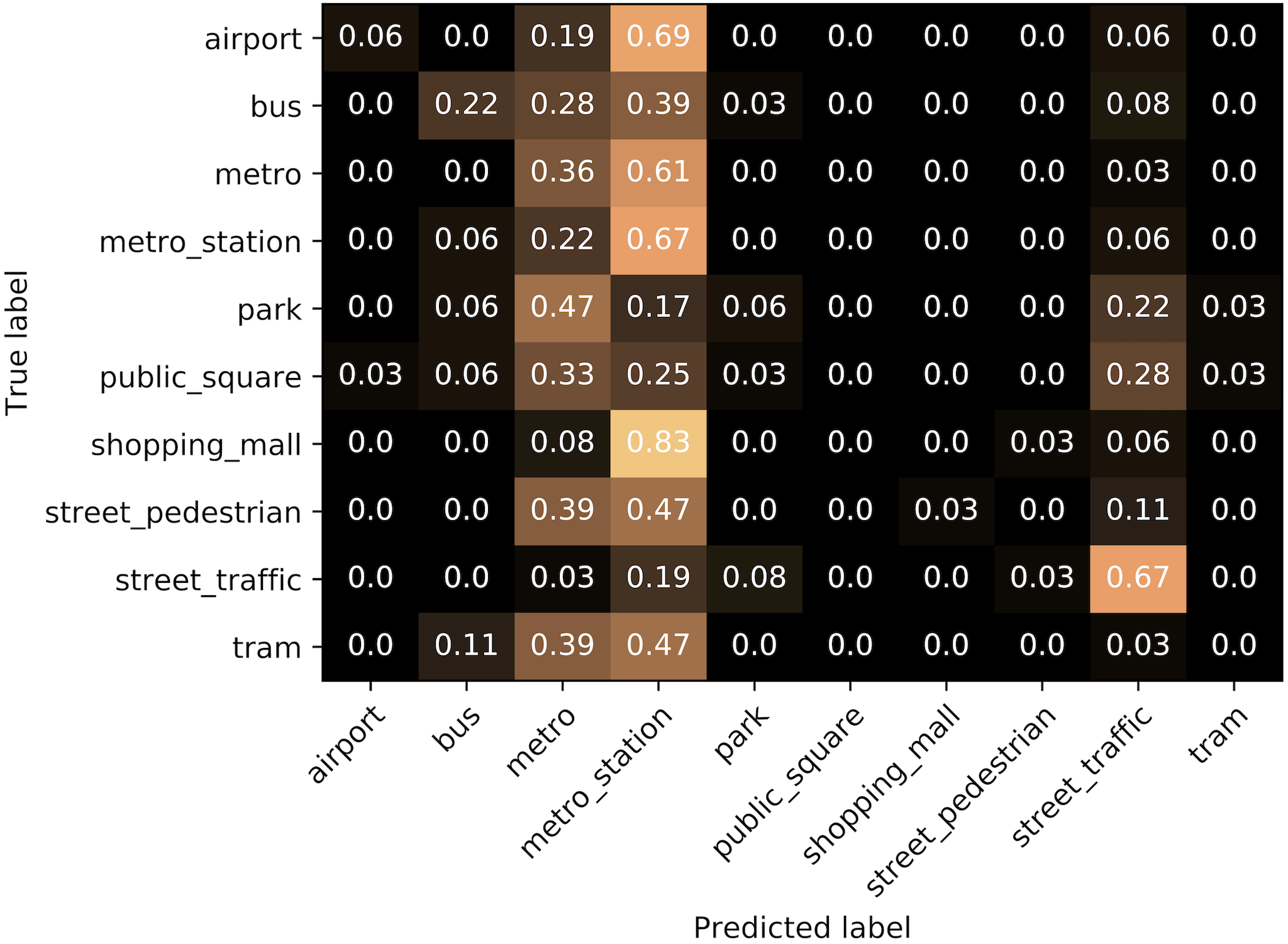
Below you can see our results in the form of confusion matrices. Each row shows how many of the recordings of the acoustic scene indicated at left, are classified as recordings from the acoustic scenes indicated above the matrix. The numbers are normalized to [0, 1] and the higher the better. The first confusion matrix shows the results when we use M_S(X_T), i.e. the non adapted model, and the second when we use M_T(X_T), i.e. the adapted model.

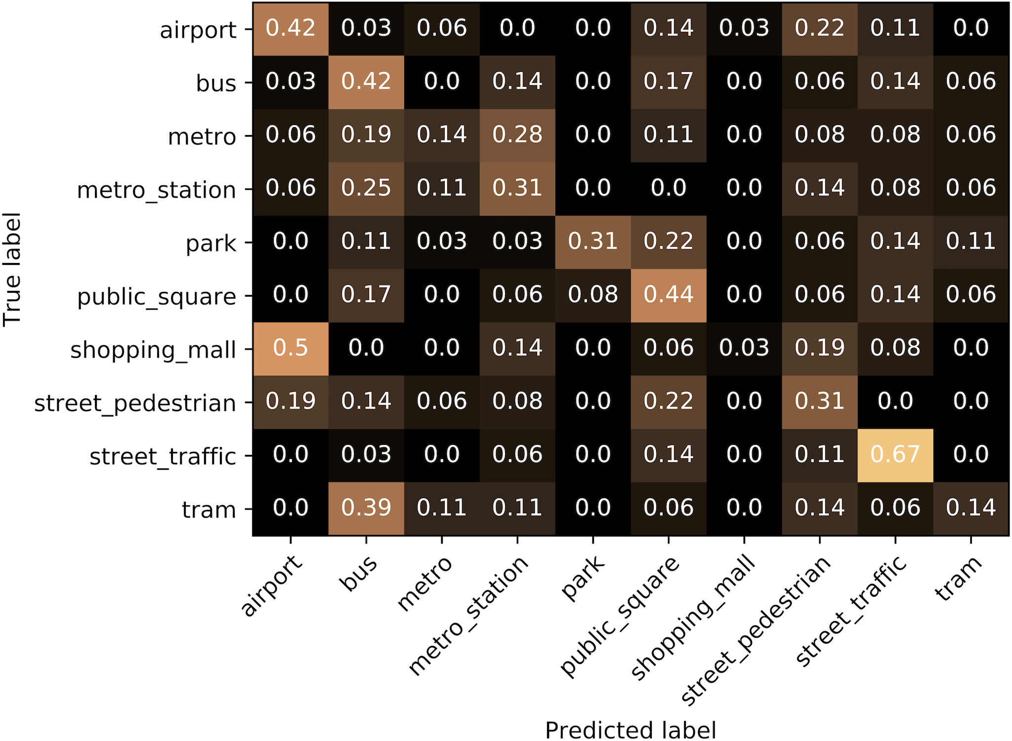Confusion matrix for the non-adapted model.	Confusion matrix for the adapted model.