No Title

Mathematical modelling constitutes an integral part of methodological concepts in the physical sciences. The basic mathematical models of science and technology have the form of differential and/or integral equations, typically expressing some kind of conservation laws. Depending on the level of idealization these models can be either linear or non-linear. Linear systems form the lowest level in the physical modelling hierarchy. In many engineering disciplines this level of sophistication has been adequate for the basis of decision-making processes in the design. However, tightening of the requirements for safety and reliability of engineering products can make the assumption of linearity insufficient.

One typical phenomenon of non-linear problems is bifurcation, which is a change in the number of solutions when one or several parameters controlling the system vary. Bifurcation thus changes the behaviour of the system even to a very dramatic extent. This birth of a new form, morphogeneses, is also a manifestation of some kind of symmetry, which is broken at the bifurcation. In a sense, the bifurcation introduces history into the model, thus implying both deterministic and probabilistic elements in it. In the neighbourhood of bifurcation small fluctuations or imperfections play an essential role in the behaviour of the system. Thus, bifurcation phenomena are intimately related to the question of structural stability which in this context has to be understood in the sense which it has in the catastrophe theory. As expressed by Prigogine: ``The concept of structural stability seems to express in the most compact way the idea of innovation, the appearance of a new mechanism and a new species, which were initially absent in the system.'' For an artistic impression of such a morphogenesis see figure 1 and a technical example, compressed plate in figure 2.

**Figure 1:** Maurits Cornelis Esher (1898-1972): Metamorphose II, woodcut 1938-1940.
$\includegraphics*[width=13cm]{MetamorphoseIILg.ps}$

Figure 2: Numerical example of mode changing.

	$\includegraphics*[width=7cm]{prebuck.ps}$
$\begin{picture}(78,60) % % SS plate aspect ratio sqrt(2) % \put(10,5){\circle*{1... ...} \put(76,25){\vector(-1,0){7}} \put(0,26){$P$ } \put(74,26){$P$ } \end{picture}$	$\includegraphics*[width=7cm]{mode1.ps}$
	$\includegraphics*[width=7cm]{mode2.ps}$
$\includegraphics*[width=7cm]{f-w.ps}$	$\includegraphics*[width=7cm]{mode3.ps}$

The bifurcation phenomenon has been known for a very long time in the physical sciences. However, bifurcation problems have usually been considered separately in different fields of physics and engineering and a unified mathematical theory, called catastrophe or singularity theory, is only thirty years old, originating from René Thom's Stabilité Structurelle et Morphogénèse published in 1972. The methods of singularity or catastrophe theory can answer the following three important and basic questions:

It should be mentioned that singularity theory has applications in other sciences than physics too, for example chemistry, biology, sociology, psycology etc.. The life starts with bifurcations.

Except in some trivial cases, analytical solution of non-linear systems is impossible. Therefore numerical approximate solution methods are necessary in order to get an insight into the phenomena being modelled. The main numerical procedures to discretize the governing partial differential equation systems are the finite difference and the finite element methods. Application of these methods results in a large non-linear algebraic equation system the solution of which can require enormous computer resources. Therefore, in addition to reliability, the numerical solution procedures have to be efficient.

Numerical solution of non-linear equations has a long history. A common iterative procedure bears the name of Newton or Newton-Raphson but there exists many names which could be credited either before Newton's time or later. The general idea of solving an equation by improving an estimate of a solution by adding a correction term had been in use in many cultures millenia prior to this time. Certain ancient Greek and Babylonian methods for extracting roots have this form, as do some methods of Arabic algebraist from at least the time at the beginning of this millenium.

Solution of parametrized non-linear equation system means construction of the solution (equilibrium) surface, the dimension of which is the dimension of the parameter space. In most practical computations the dimension of the parameter space equals to unity. Thus, the problem is reduced in tracing a curve in a N+1 dimensional Euclidean space, where N is the dimension of the discretized mathematical problem, which can be very large. At present day supercomputers models larger than 100 million unknowns can be solved, even a single PC can handle problems over 100000 unknowns very efficiently.

The aim of the present work has been to develop and implement general procedures for the analysis of non-linear discretized structural models. Special emphasis is given to the handling of critical points and solution of the post-critical behaviour. Even though the presentation mainly concentrates on analysis of solid bodies, many of the developed procedures are applicable to heat transfer and fluid flow problems, too.

For having a closer look to the problem, the figure 3 shows some equilibrium curves, which are assumed to represent the exact solutions of certain discretized models. From this figure critical points, like limit and bifurcation points can easily be located. However, the numerical reality does not look as good as these diagrams. The output of a typical continuation can look like the set of dots drawn in figure 4. It requires imagination and confidence to draw a good diagram from the few points the computer gives us; the many difficulties are seldom mentioned in the papers, see e.g. figure 5.

Stability is a classical subject in structural mechanics. The early considerations restricted mainly to the determination of stability limit from a neutral equilibrium state. It became soon evident that the bifurcation load itself is not always sufficient in describing the critical behaviour of a structure. A classical example is the discrepancy between the theoretical bifurcation load and the experimentally observed critical loads for compressed cylindrical shells.

A general theory of post-buckling phenomena of elastic structures was developed during the second world war by Koiter who explained the paradox by imperfection sensitivity which is induced by interacting buckling modes. Koiter's initial post-buckling theory is asymptotic in nature, thus the range of validity can be rather small. However, combining the asymptotic approach to a general continuation algorithm may provide some useful information to the analyst and in addition it can be used as a branch switching procedure. This approach is applied to multi-mode problems in the present study.

Nevertheless, the cylindrical shell still challenges this approach. Figure 7 shows the lowest buckling mode of a compressed cylinder, but it should be remembered that more than 100 eigenmodes with critical loads diffring less than 4 % clusteres the lowest one.

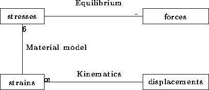
The third major topic in this thesis is related to kinematical equations. As it is shown in figure 6 the governing equation system comprises three types of equations expressing equilibrium, material behaviour and kinematical relations. Since equilibrium- and kinematical equations are adjoint to each other, non-linearity can enter into the model from two sources: from non-linear kinematics and/or non-linear material models.

In stability analysis the non-linearity is geometrical in nature, and in many cases it can be adequately discribed by models where the local strains are assumed to be small but the rotations are finite. Since 3-dimensional rotations do not belong to a linear configuration space, derivation for the linearized weak form of the non-linear equilibrium equations is not a trivial task. If the incremental rotations are assumed to be small, but finite, some simplifications can be done. In this work necessary requirements for truncation of the series expansion of the rotation tensor has been investigated.

**Figure 6:** The ``holy trinity'' of mechanics.
$\begin{figure}\begin{center} \setlength{\unitlength}{1mm} \begin{picture} (95,4... ...(1,0){45}} \put(65,3.5){\vector(-1,0){45}} \end{picture}\end{center}\end{figure}$

Figure 7: Compressed cylindrical shell with clamped ends: (a) buckling mode corresponding to the lowest critical eigenvalue and (b) the list of 100 lowest critical loads with respect to the classical buckling load. The model consists of 18000 quadrilateral 4-node elements resulting in 107281 unknowns.

(a)

(b)

$\includegraphics*[width=7cm]{cm1b.ps}$

mode	critical load	mode	critical load
1	1.0057616	51	1.0290370
2	1.0057616	52	1.0290370
3	1.0057766	53	1.0306942
4	1.0057766	54	1.0306942
5	1.0081014	55	1.0308432
6	1.0081014	56	1.0308432
7	1.0088316	57	1.0318304
8	1.0088316	58	1.0318304
9	1.0126105	59	1.0318336
10	1.0126105	60	1.0318336
11	1.0126496	61	1.0326339
12	1.0126496	62	1.0326339
13	1.0154038	63	1.0326464
14	1.0154038	64	1.0326464
15	1.0154106	65	1.0326818
16	1.0154106	66	1.0326818
17	1.0166330	67	1.0327178
18	1.0166330	68	1.0327178
19	1.0166529	69	1.0339157
20	1.0166529	70	1.0339157
21	1.0183169	71	1.0339236
22	1.0183169	72	1.0339236
23	1.0183381	73	1.0354852
24	1.0183381	74	1.0354852
25	1.0201017	75	1.0355225
26	1.0201017	76	1.0355225
27	1.0201521	77	1.0368105
28	1.0201521	78	1.0368105
29	1.0205692	79	1.0368157
30	1.0205692	80	1.0368157
31	1.0206552	81	1.0372411
32	1.0206552	82	1.0372411
33	1.0217965	83	1.0372941
34	1.0217965	84	1.0372941
35	1.0218027	85	1.0373126
36	1.0218027	86	1.0373126
37	1.0218610	87	1.0377411
38	1.0218610	88	1.0377411
39	1.0219420	89	1.0377708
40	1.0219420	90	1.0377708
41	1.0237540	91	1.0379036
42	1.0237540	92	1.0379036
43	1.0237779	93	1.0380686
44	1.0237779	94	1.0380686
45	1.0259291	95	1.0381069
46	1.0259291	96	1.0381069
47	1.0260682	97	1.0393074
48	1.0260682	98	1.0393074
49	1.0287757	99	1.0393977
50	1.0287757	100	1.0393977